Evaluate the presence of sample level batch effects by PILOT (Subgroups of patients)
import PILOT as pl
import scanpy as sc
import pandas as pd
Reading the original Anndata:
First, we consider the original kidney single cell data. You can download the Anndata (h5ad) file from here, and place it in the Datasets folder.
adata = sc.read_h5ad('/Datasets/Kidney_ori.h5ad')
Loading the required information and computing the Wasserstein distance:
Use the following parameters to configure PILOT for your analysis (Setting Parameters):
adata: Pass your loaded Anndata object to PILOT.
emb_matrix: Provide the name of the variable in the obsm level that holds the dimension reduction (PCA representation).
clusters_col: Specify the name of the column in the observation level of your Anndata that corresponds to cell types or clusters.
sample_col: Indicate the column name in the observation level of your Anndata that contains information about samples or patients.
status: Provide the column name that represents the status or disease (e.g., “control” or “case”).
pl.tl.wasserstein_distance(
    adata,
    emb_matrix = 'X_pca',
    clusters_col = 'cell_type',
    sample_col = 'donor_id',
    status = 'disease'
    )
Patients sub-group detection by clustering the Wasserstein distance.
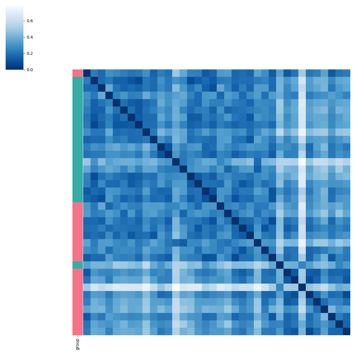
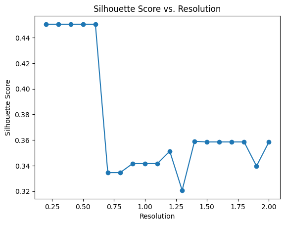
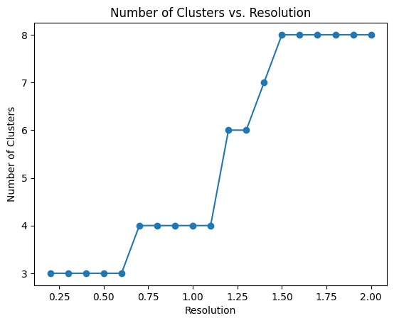
pl.pl.select_best_sil(adata, start = 0.2)
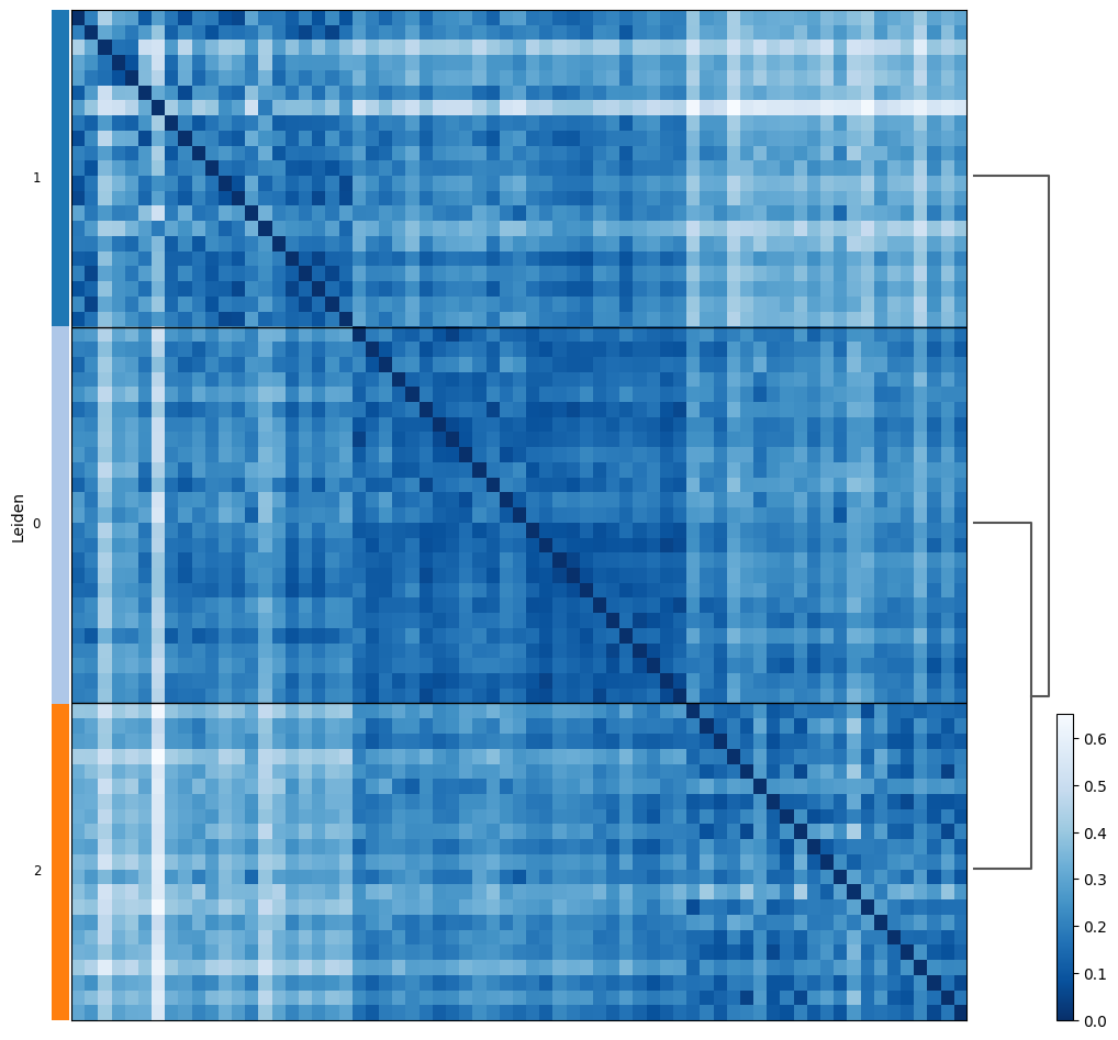
proportion_df=pl.pl.clustering_emd(adata, res = adata.uns['best_res'],show_gene_labels=False,sorter_leiden=['1','0','2'],save=True)
Evaluation of the association of estimated subgroups with experimental factor:
A very important question is if PILOT analysis is affected by experimental artefacts (location of tissues, batch processing). To evaluate this, we use ANOVA statistics and Chi-Squared correlation to check any association between any variables describing the found clusters. To run these functions, provide the sample_col as the Sample/Patient column and your interested variables. Of note, these functions only show the significant variables (p-value < 0.05).
categorical = ['BMI','hypertension','development_stage','sex','eGFR','diabetes_history','disease','tissue']
pl.tl.correlation_categorical_with_clustering(adata, proportion_df, sample_col = 'donor_id', features = categorical)
| Feature | ChiSquared_Statistic | ChiSquared_PValue | |
|---|---|---|---|
| 7 | tissue | 21.906065 | 0.001259 |
| 0 | BMI | 18.291352 | 0.005544 |
| 6 | disease | 10.600704 | 0.031438 |
Similarly, you can do the same analysis for numerical variables.
numeric = ['degen.score','aStr.score','aEpi.score','matrisome.score','collagen.score','glycoprotein.score','proteoglycan.score']
pl.tl.correlation_numeric_with_clustering(adata, proportion_df, sample_col = 'donor_id', features = numeric)
| Feature | ANOVA_F_Statistic | ANOVA_P_Value |
|---|
We observe that there is a clear association between the sub-clusters and the origin of the biopsies. This is not surprising as PILOT uses cellular composition information, as samples at distinct regions do have distinct cells.
To double check these results, one can of course plot the heatmap of clusters by showing the variables with ‘clinical_variables_corr_sub_clusters’ function.
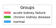
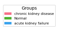
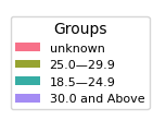
Disease
pl.tl.clinical_variables_corr_sub_clusters(adata,sorter_order=['1','0','2'],sample_col='donor_id',feature='disease',proportion_df=proportion_df,figsize_legend=(1,1))
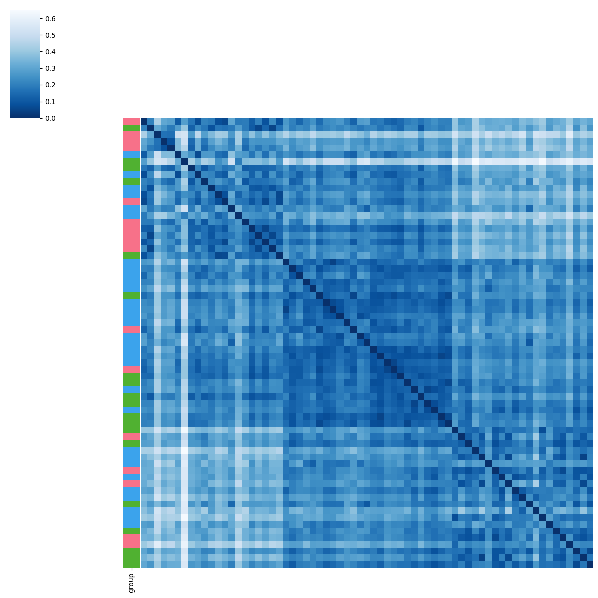
Tissue
pl.tl.clinical_variables_corr_sub_clusters(adata,sorter_order=['1','0','2'],sample_col='donor_id',feature='tissue',proportion_df=proportion_df,figsize_legend=(1,1))
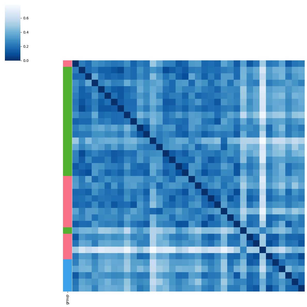
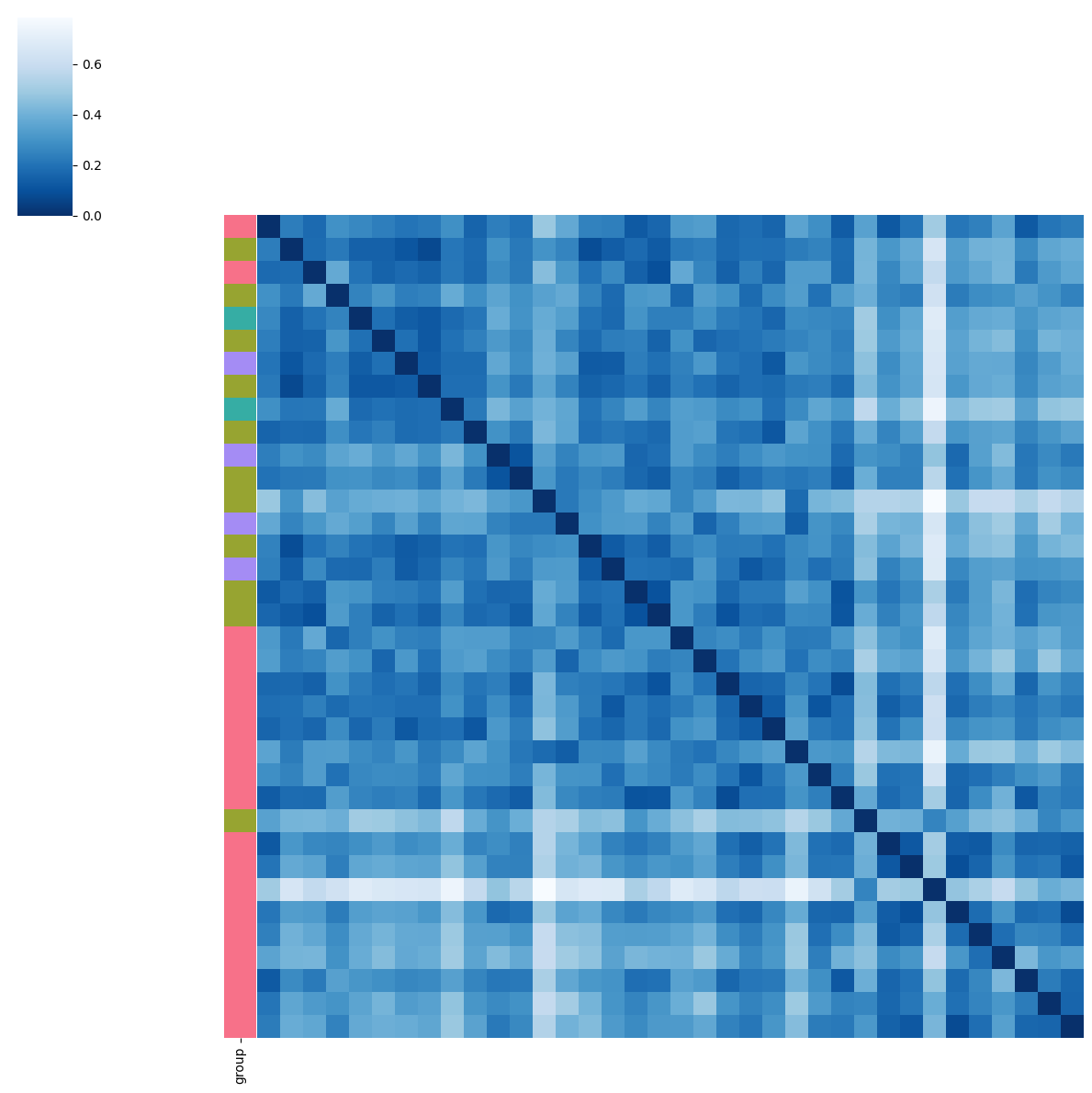
BMI
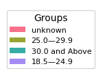
pl.tl.clinical_variables_corr_sub_clusters(adata,sorter_order=['1','0','2'],sample_col='donor_id',feature='BMI',proportion_df=proportion_df,figsize_legend=(1,1))

Filtering of samples
Therefore, we only focus on biopsies from sample locationn ‘kidney’, which were used in our benchmarking. You can download the Anndata (h5ad) file from here, and place it in the Datasets folder.
adata_filtered=sc.read_h5ad('/Datasets/Kidney.h5ad')
pl.tl.wasserstein_distance(
    adata_filtered,
    emb_matrix = 'X_pca',
    clusters_col = 'cell_type',
    sample_col = 'donor_id',
    status = 'disease'
    )
Run the same functions for the filtered data.
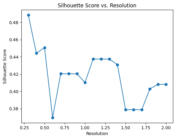
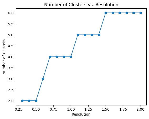
pl.pl.select_best_sil(adata_filtered, start = 0.3)
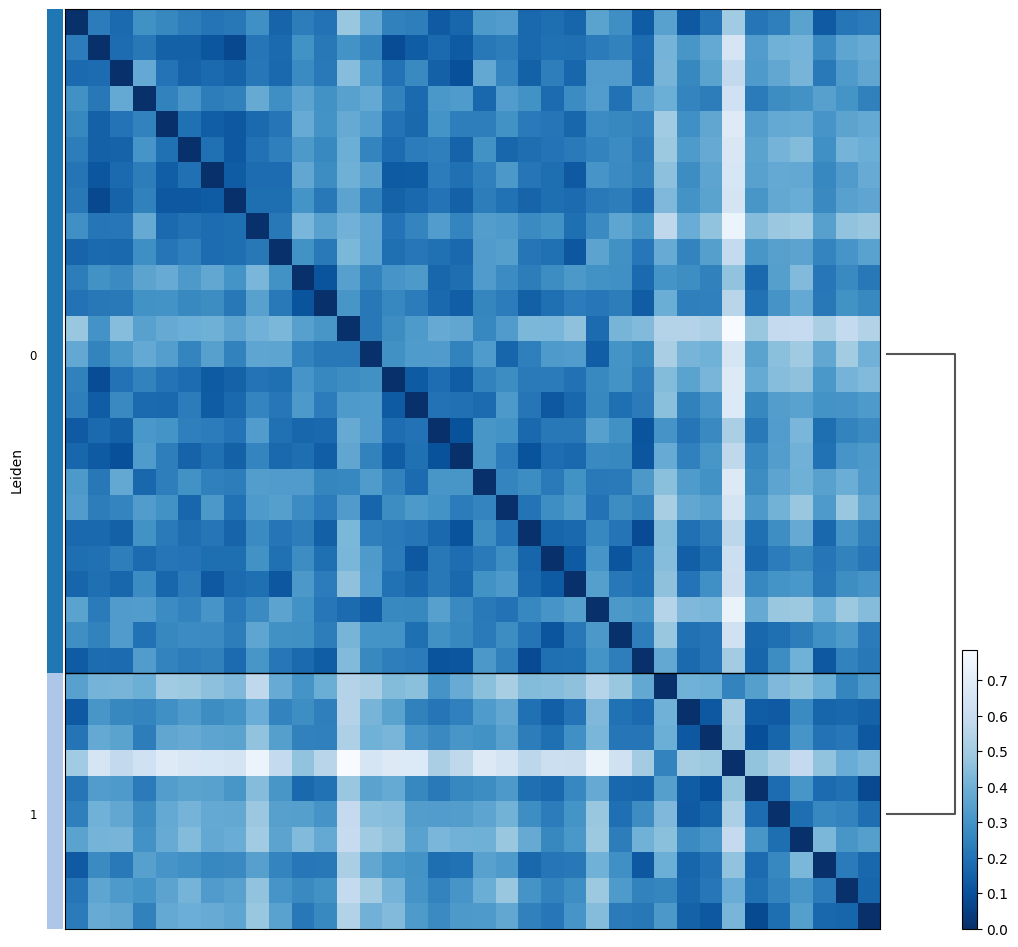
proportion_df=pl.pl.clustering_emd(adata_filtered, res = adata_filtered.uns['best_res'],show_gene_labels=False,sorter_leiden=['0','1'],save=True)
We next recheck the association of variables with the estimated sub-clusters.
pl.tl.correlation_categorical_with_clustering(adata_filtered,proportion_df,sample_col= 'donor_id', features = categorical)
| Feature | ChiSquared_Statistic | ChiSquared_PValue | |
|---|---|---|---|
| 6 | disease | 17.488757 | 0.000159 |
| 5 | diabetes_history | 6.784615 | 0.009195 |
| 0 | BMI | 7.857195 | 0.049057 |
In the data we observed that the true label (disease) has the highest association followed by Diabetes History and BMI.
We can show the distribution of variables in the found clusters:
Disease
meta=adata_filtered.obs[['diabetes_history','BMI','donor_id','disease']]
meta = meta.drop_duplicates(subset='donor_id').rename(columns={'donor_id': 'sampleID'})
proportion=proportion_df[['Predicted_Labels','sampleID']].merge(meta,on='sampleID')
contingency_table = pd.crosstab(proportion['disease'], proportion['Predicted_Labels'],values=proportion['sampleID'], aggfunc=pd.Series.nunique, margins=True, margins_name='Total Unique Patients')
# Display the contingency table
contingency_table
| Predicted_Labels | 0 | 1 | Total Unique Patients |
|---|---|---|---|
| disease | |||
| Normal | 17.0 | 1.0 | 18 |
| acute kidney failure | NaN | 5.0 | 5 |
| chronic kidney disease | 9.0 | 4.0 | 13 |
| Total Unique Patients | 26.0 | 10.0 | 36 |
BMI
contingency_table = pd.crosstab(proportion['BMI'], proportion['Predicted_Labels'],values=proportion['sampleID'], aggfunc=pd.Series.nunique, margins=True, margins_name='Total Unique Patients')
contingency_table
| Predicted_Labels | 0 | 1 | Total Unique Patients |
|---|---|---|---|
| BMI | |||
| 18.5—24.9 | 2.0 | NaN | 2 |
| 25.0—29.9 | 10.0 | 1.0 | 11 |
| 30.0 and Above | 4.0 | NaN | 4 |
| unknown | 10.0 | 9.0 | 19 |
| Total Unique Patients | 26.0 | 10.0 | 36 |
Diabetes history
contingency_table = pd.crosstab(proportion['diabetes_history'], proportion['Predicted_Labels'],values=proportion['sampleID'], aggfunc=pd.Series.nunique, margins=True, margins_name='Total Unique Patients')
# Display the contingency table
contingency_table
| Predicted_Labels | 0 | 1 | Total Unique Patients |
|---|---|---|---|
| diabetes_history | |||
| No | 17 | 1 | 18 |
| Yes | 9 | 9 | 18 |
| Total Unique Patients | 26 | 10 | 36 |
To double check these results, one can of course plot the heatmap of clusters by showing the variables with ‘clinical_variables_corr_sub_clusters’ function.
Disease
pl.tl.clinical_variables_corr_sub_clusters(adata_filtered, sorter_order=['0','1'],sample_col='donor_id',feature= 'disease',proportion_df = proportion_df,figsize_legend=(1,1))
BMI
pl.tl.clinical_variables_corr_sub_clusters(adata_filtered, sorter_order = ['0','1'],sample_col = 'donor_id',feature = 'BMI',proportion_df = proportion_df,figsize_legend=(1,1))
Diabetes_history
pl.tl.clinical_variables_corr_sub_clusters(adata_filtered, sorter_order = ['0','1'],sample_col = 'donor_id',feature = 'diabetes_history',proportion_df = proportion_df,figsize_legend=(1,1))