Patients sub-group detection by PILOT
In this tutorial, we are using single-cell data from pancreatic ductal adenocarcinomas to find sub-groups of patients using clustering of W distances. And then we rank the cells/genes based on clustering results.
You can download the Anndata (h5ad) file for this tutorial from here and place it in the Datasets folder.
import PILOT as pl
import scanpy as sc
Reading Anndata
adata = sc.read_h5ad('Datasets/PDAC.h5ad')
Loading the required information and computing the Wasserstein distance:
Use the following parameters to configure PILOT for your analysis (Setting Parameters):
adata: Pass your loaded Anndata object to PILOT.
emb_matrix: Provide the name of the variable in the obsm level that holds the dimension reduction (PCA representation).
clusters_col: Specify the name of the column in the observation level of your Anndata that corresponds to cell types or clusters.
sample_col: Indicate the column name in the observation level of your Anndata that contains information about samples or patients.
status: Provide the column name that represents the status or disease (e.g., “control” or “case”).
pl.tl.wasserstein_distance(
    adata,
    emb_matrix='X_pca',
    clusters_col='cell_types',
    sample_col='sampleID',
    status='status'
    )
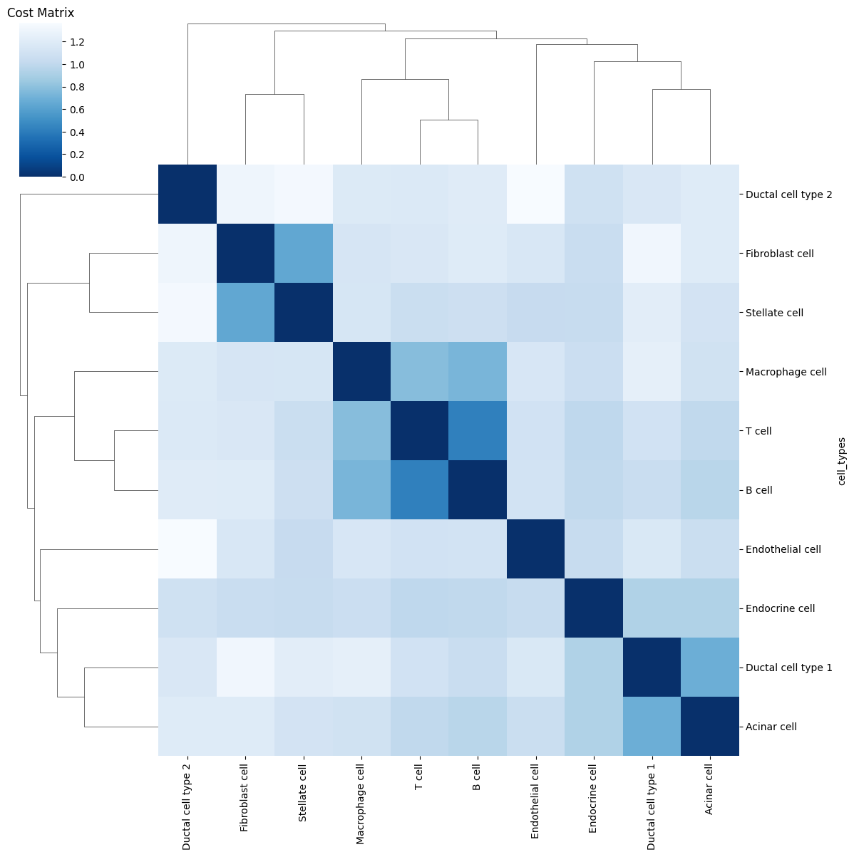
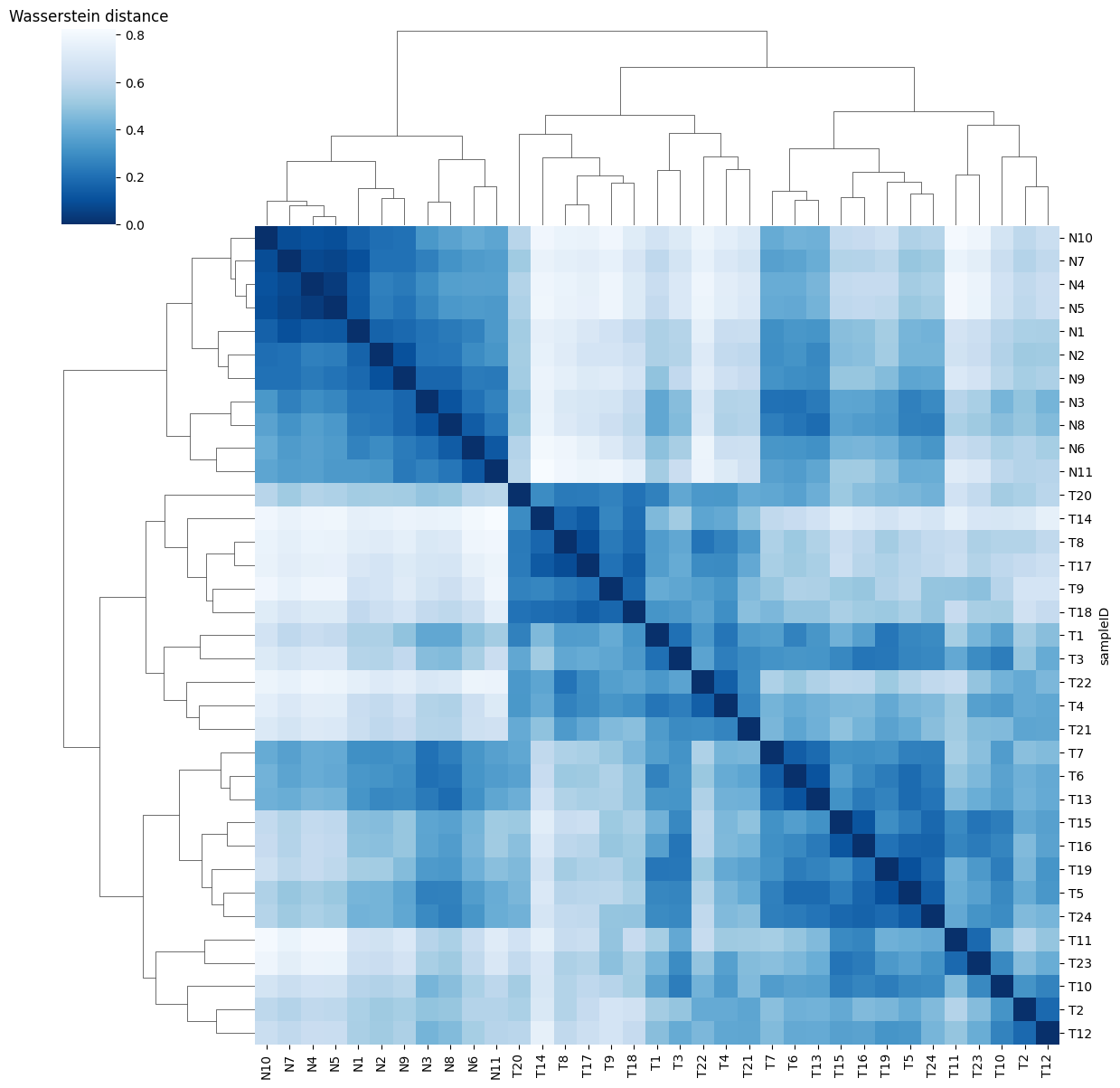
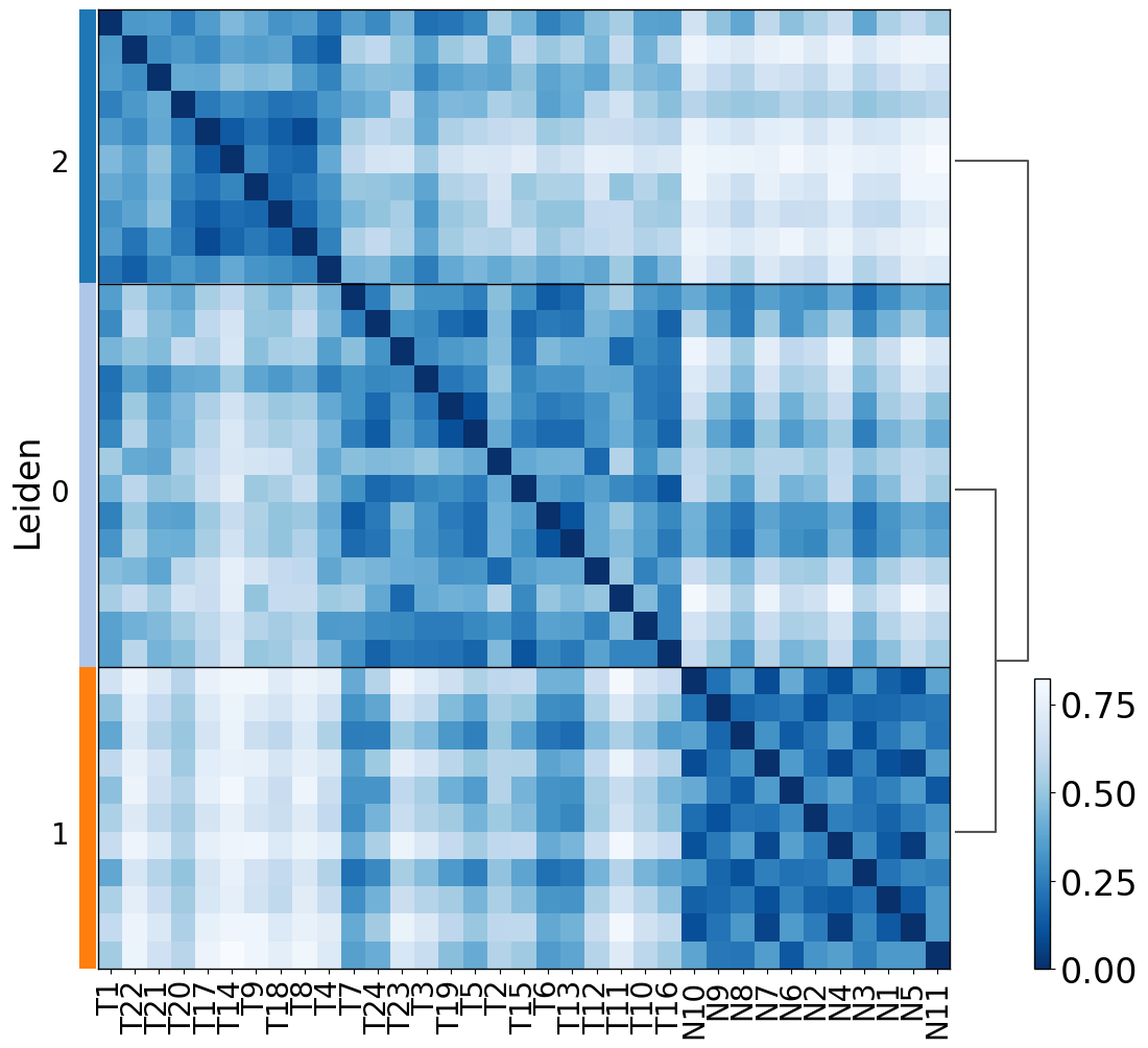
Ploting the Cost matrix and the Wasserstein distance:
pl.pl.heatmaps(adata)
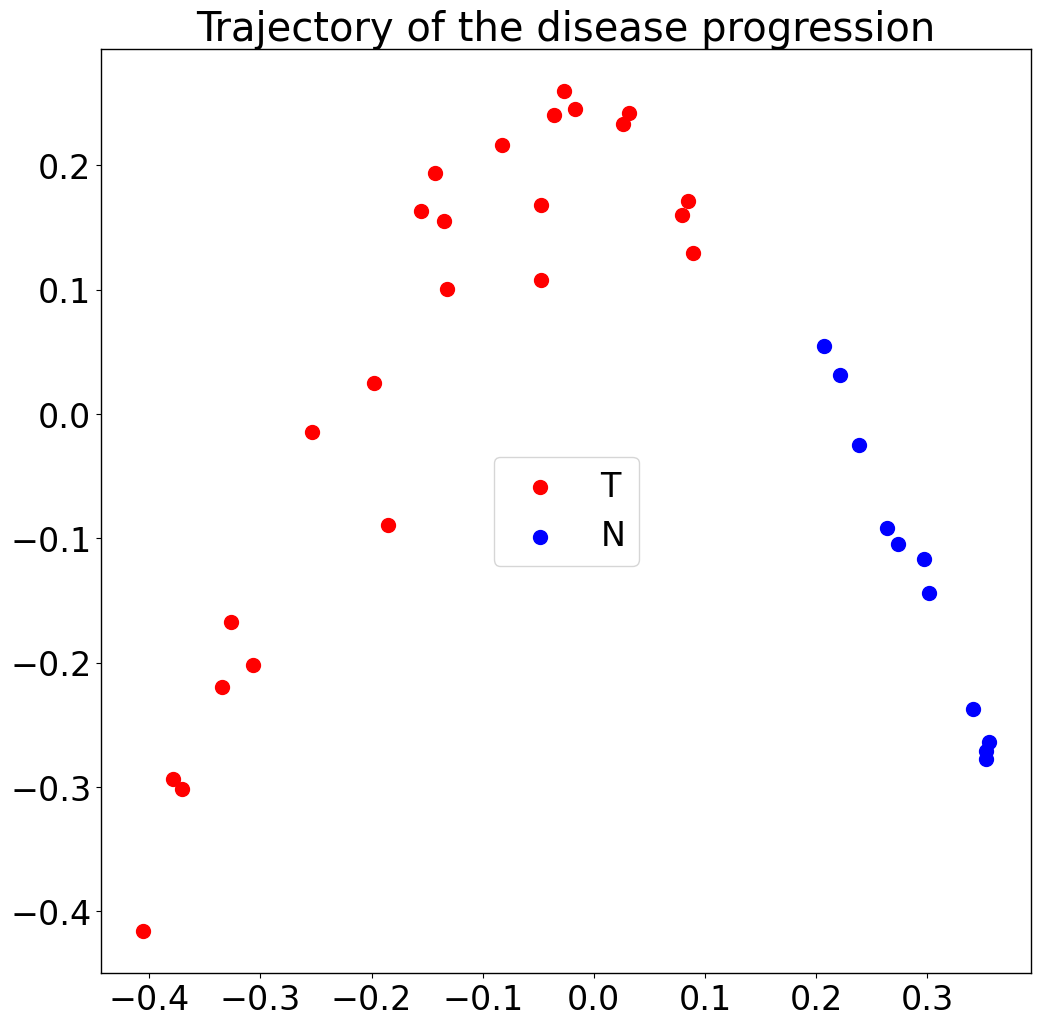
Trajectory:
pl.pl.trajectory(adata, colors = ['red','Blue'])
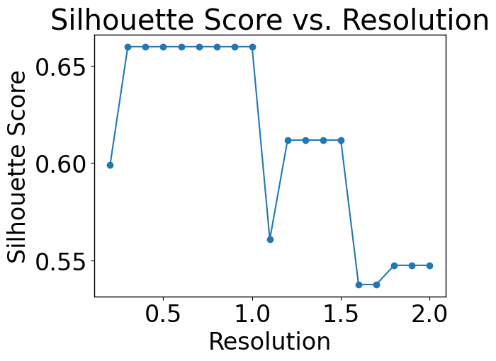
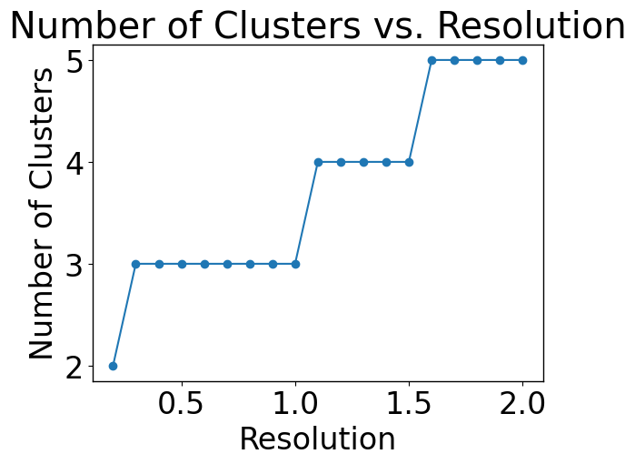
In this section, we should find the optimal number of clusters.
pl.pl.select_best_sil(adata)
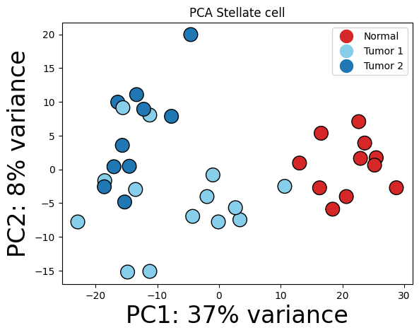
Patients sub-group detection by clustering EMD.
proportion_df=pl.pl.clustering_emd(adata, res = adata.uns['best_res'])
proportion_df.loc[proportion_df['Predicted_Labels'] == '0', 'Predicted_Labels'] = 'Tumor 1'
proportion_df.loc[proportion_df['Predicted_Labels'] == '1', 'Predicted_Labels'] = 'Normal'
proportion_df.loc[proportion_df['Predicted_Labels'] == '2', 'Predicted_Labels'] = 'Tumor 2'
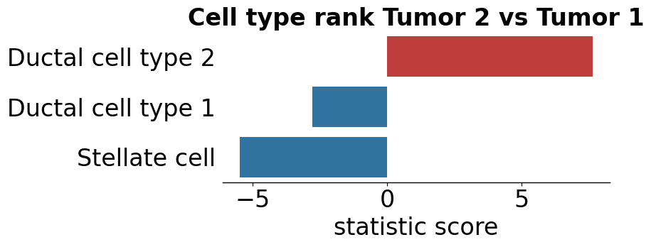
Cell-type selection.
Based on the adjusted p-value threshold you consider, you can choose how statistically significant the cell types you want to have.
pl.pl.cell_type_diff_two_sub_patient_groups(
    proportion_df,
    proportion_df.columns[0:-2],
    group1 = 'Tumor 2',
    group2 = 'Tumor 1',
    pval_thr = 0.05,
    figsize = (15, 4)
    )
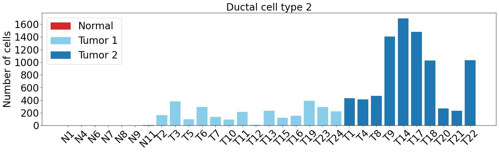
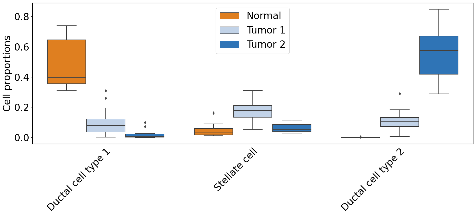
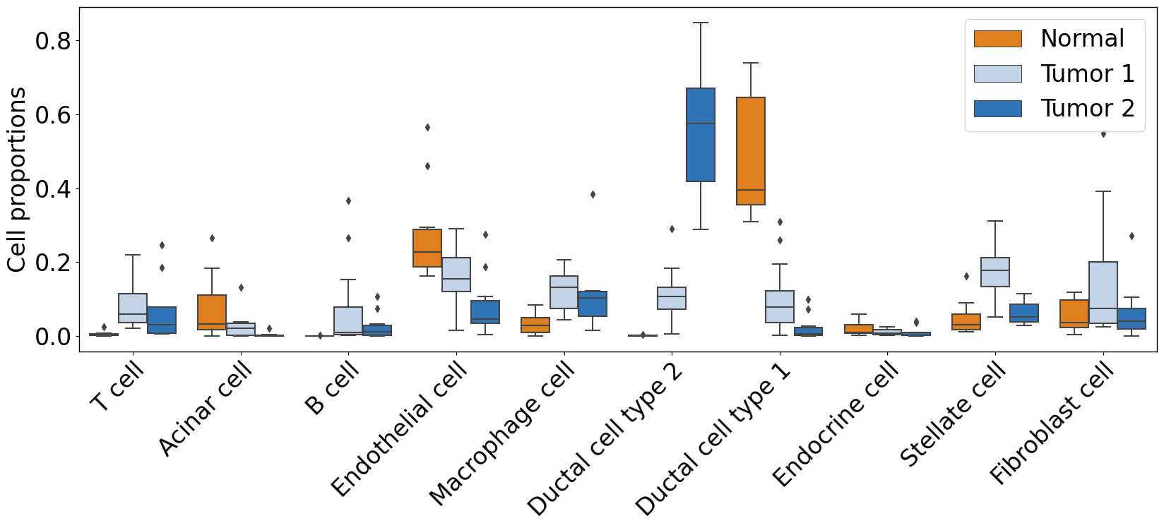
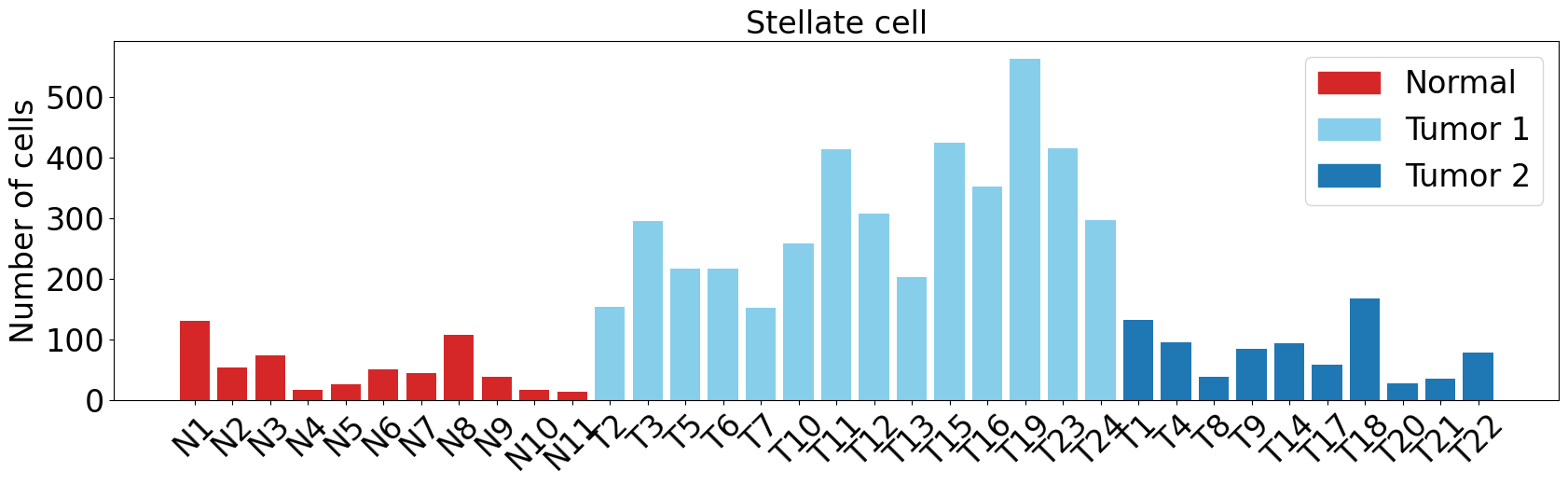
pl.pl.plot_cell_types_distributions(
    proportion_df,
    cell_types = ['Stellate cell','Ductal cell type 2','Ductal cell type 1'],
    figsize = (17,8),
    label_order = ['Normal', 'Tumor 1', 'Tumor 2'],
    label_colors = ['#FF7F00','#BCD2EE','#1874CD']
    )
pl.pl.plot_cell_types_distributions(
    proportion_df,
    cell_types = list(proportion_df.columns[0:-2]),
    figsize = (17,8),
    label_order = ['Normal', 'Tumor 1', 'Tumor 2'],
    label_colors = ['#FF7F00','#BCD2EE','#1874CD']
    )
Differential expression analysis
Note:
#pl.tl.install_r_packages()
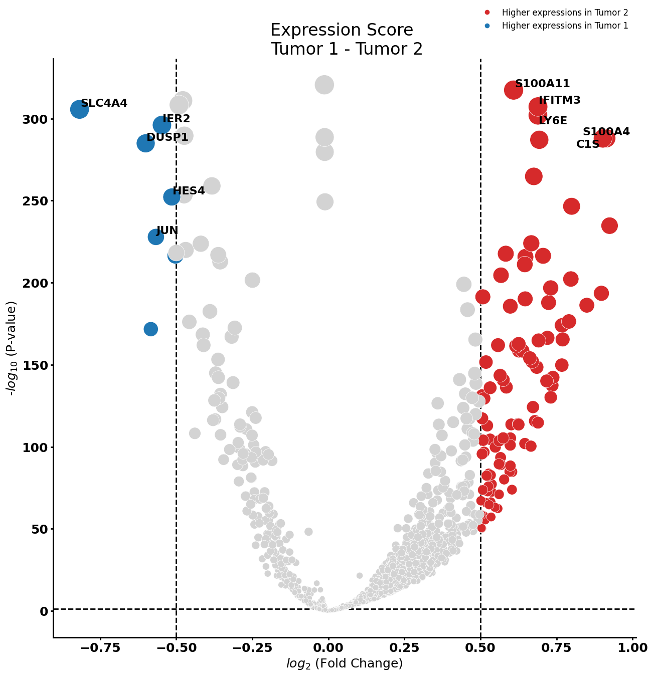
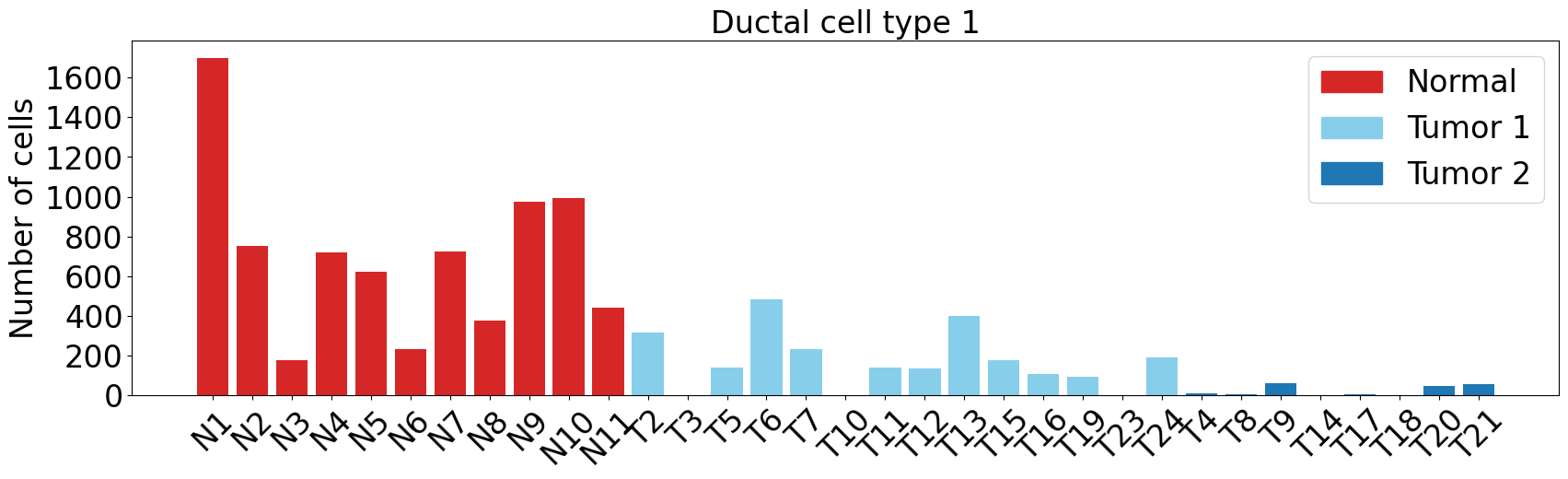
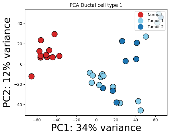
Ductal cell type 1
You can run this function for your own data, and it automatically extracts the gene expressions for each cell type (“2000 highly variable genes). In case you want all/more genes, please change the “highly_variable_genes_” or “n_top_genes” parameters.
cell_type = "Ductal cell type 1"
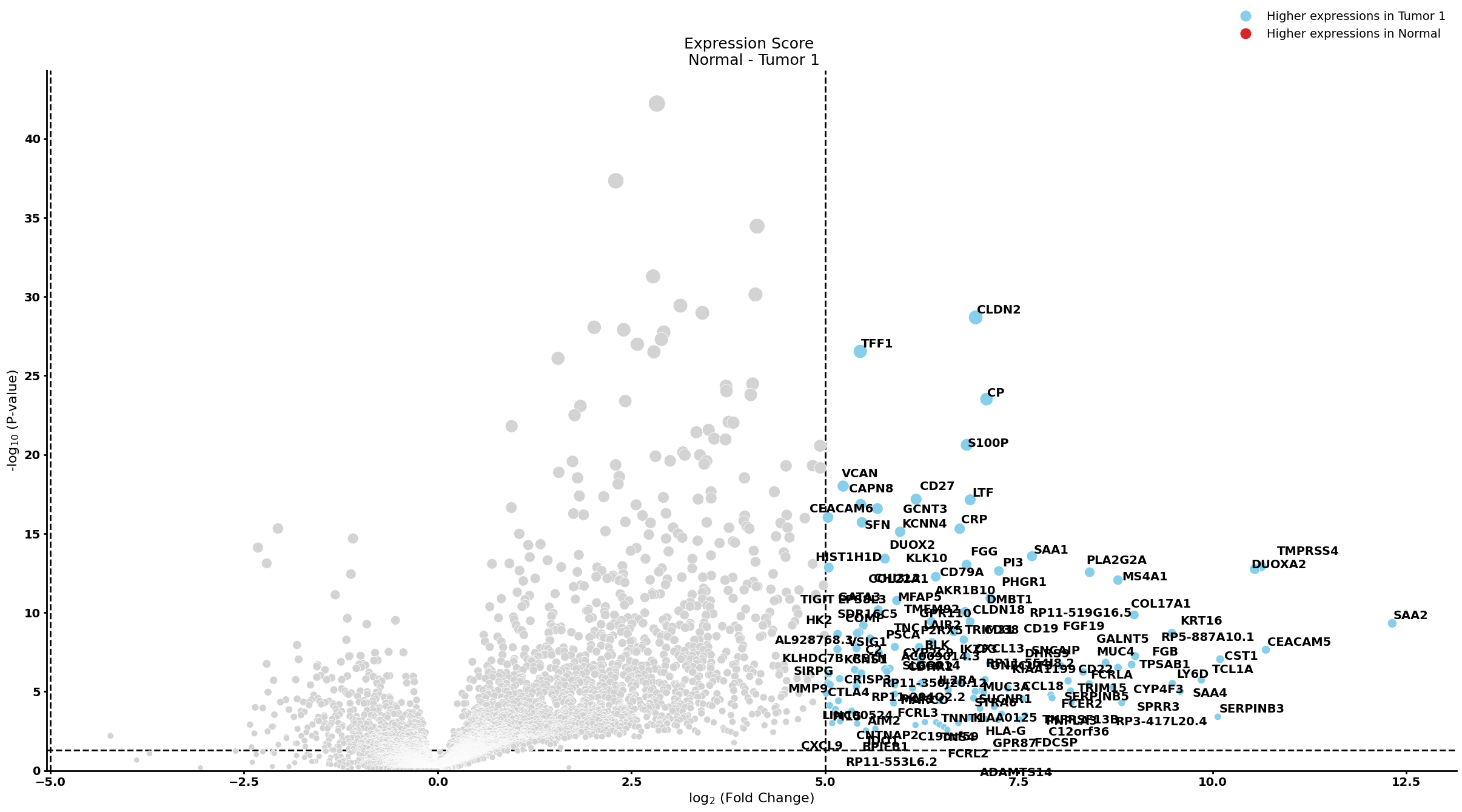
pl.tl.compute_diff_expressions(
adata,
cell_type,
proportion_df,
fc_thr = 0.5,
pval_thr = 0.05,
group1 = 'Tumor 1',
group2 = 'Tumor 2',
sample_col = 'sampleID',
col_cell = 'cell_types',
)
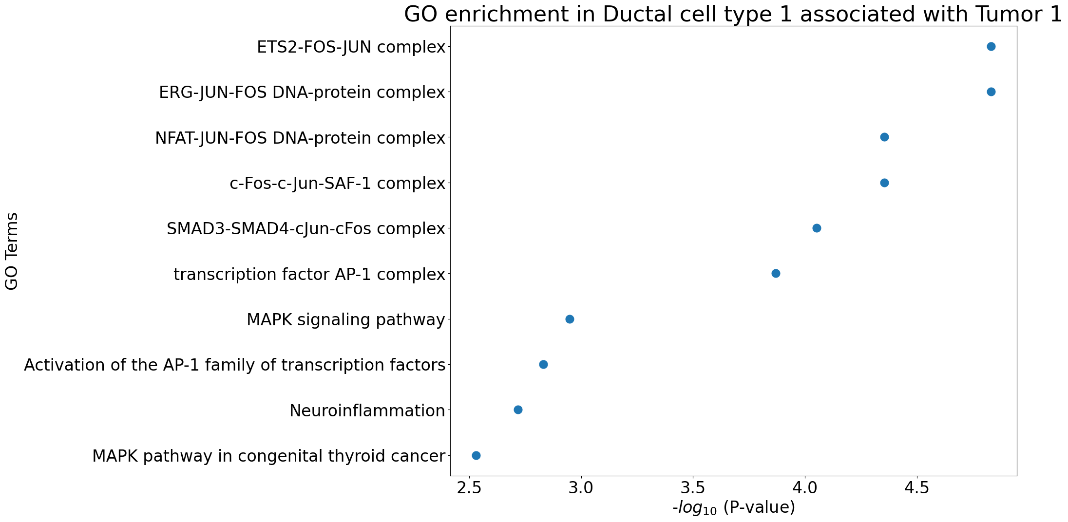
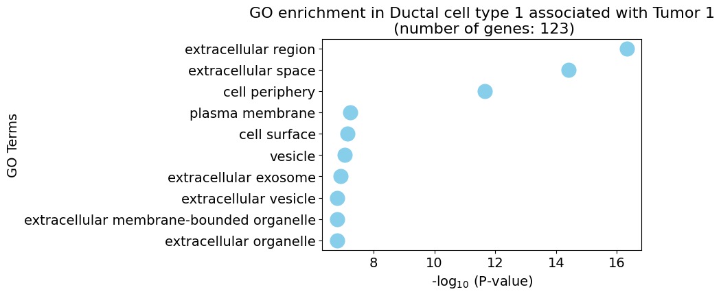
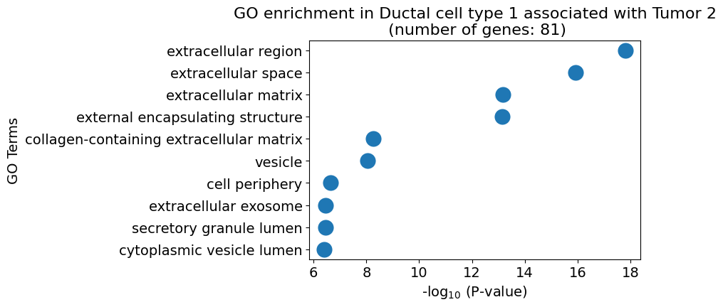
Gene Ontology analysis
pl.pl.gene_annotation_cell_type_subgroup(
    cell_type = cell_type,
    group = 'Tumor 1',
    num_gos = 10
    )
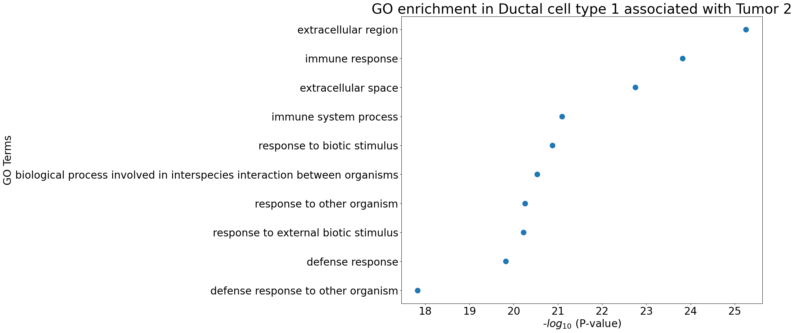
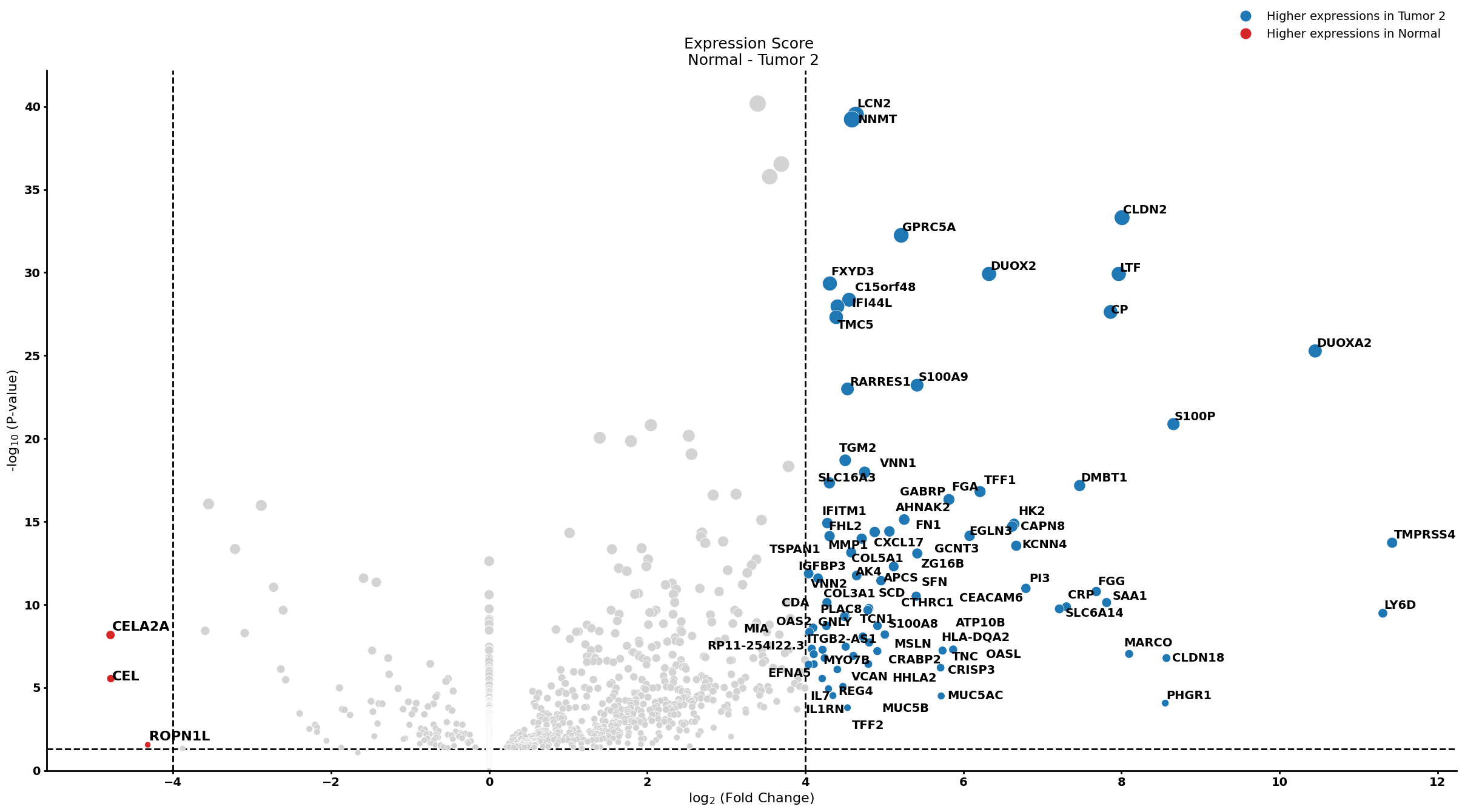
pl.pl.gene_annotation_cell_type_subgroup(
    cell_type = cell_type,
    group = 'Tumor 2',
    num_gos = 10
    )
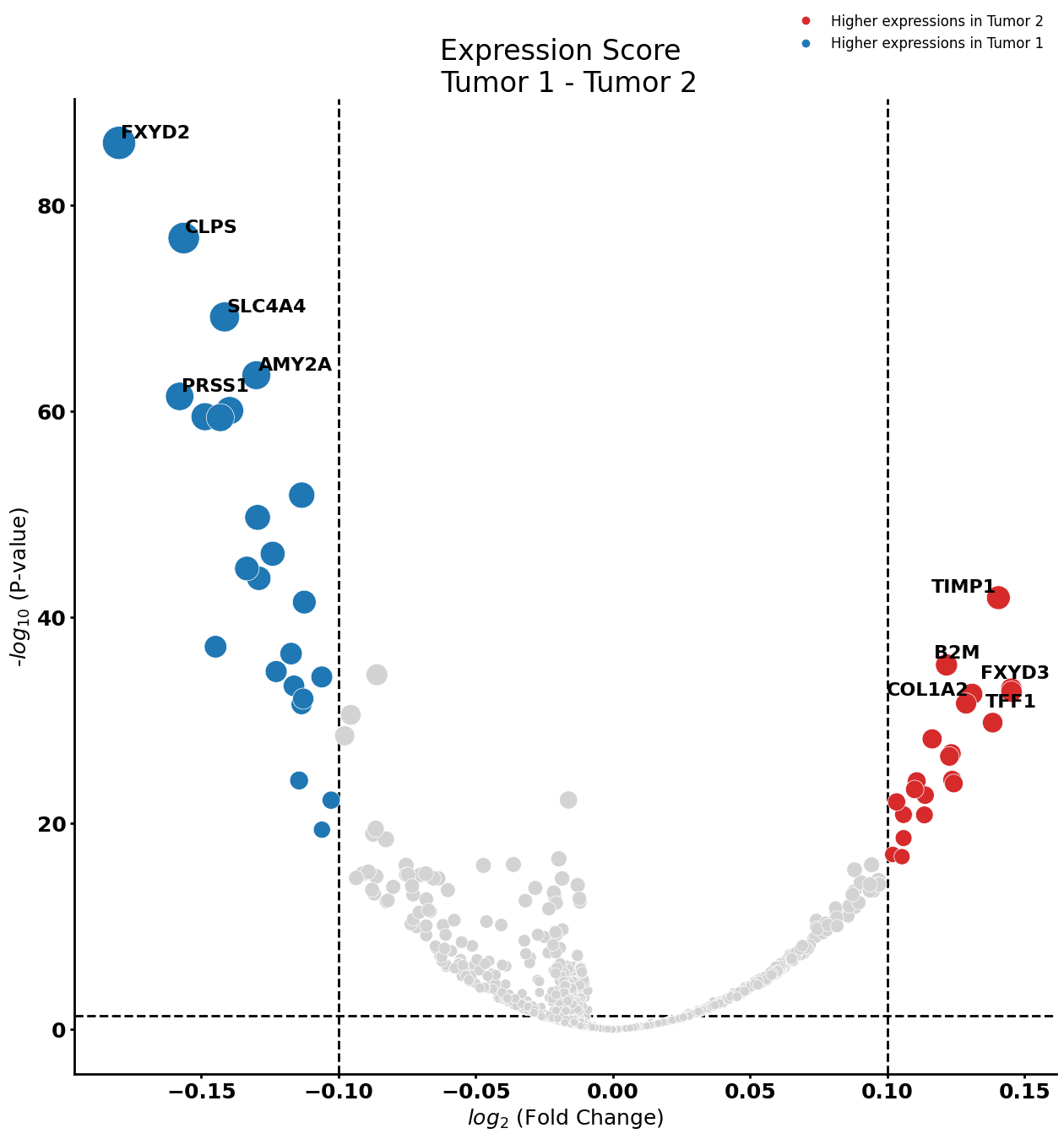
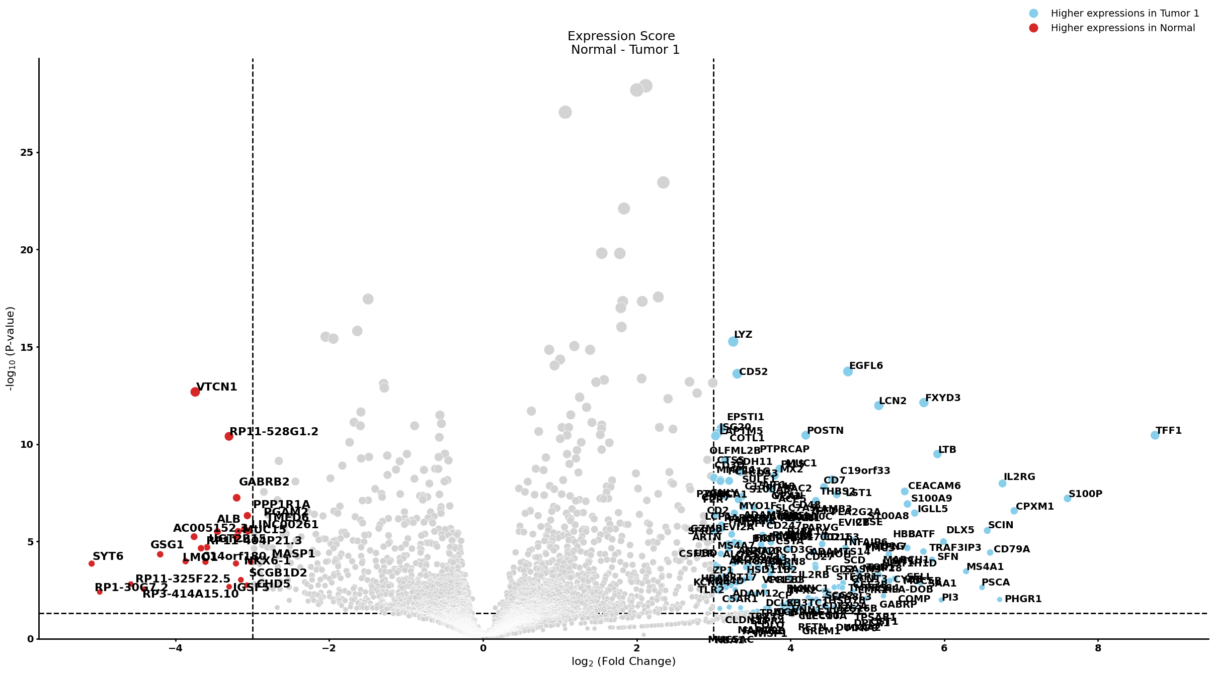
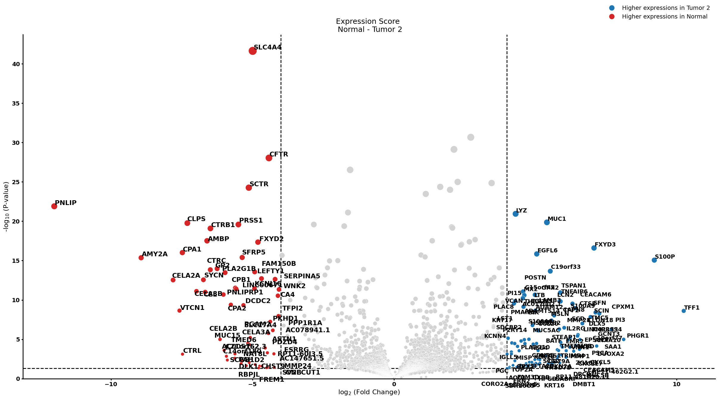
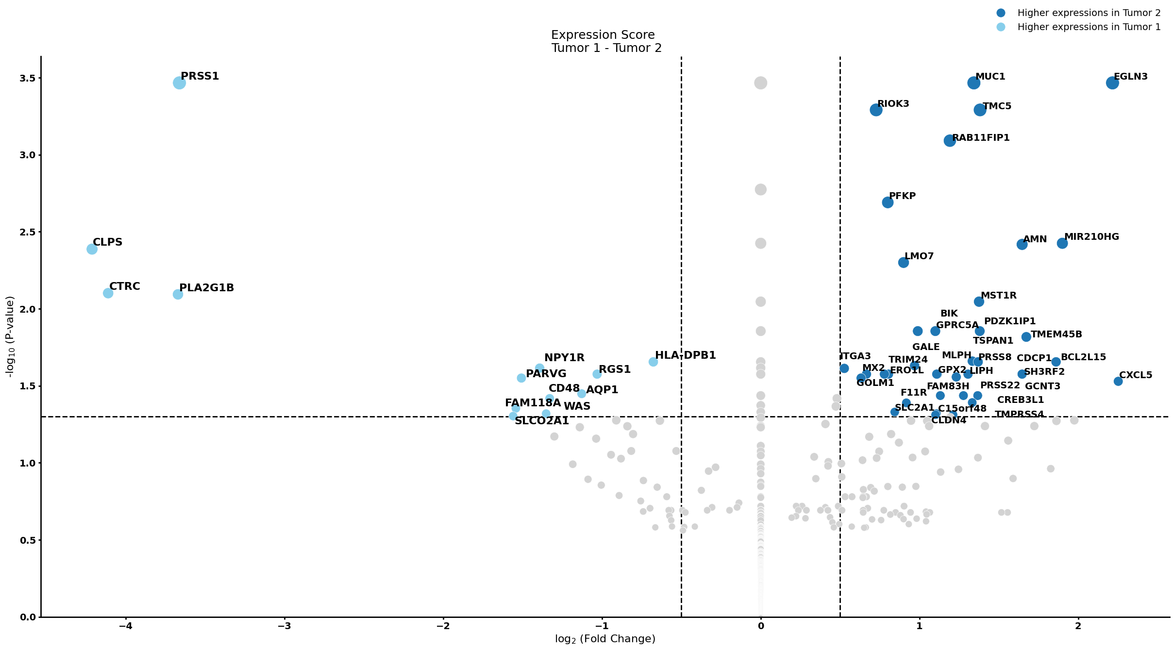
Stellate cell
cell_type = "Stellate cell"
pl.tl.compute_diff_expressions(
    adata,
    cell_type,
    proportion_df,
    fc_thr = 0.1,
    pval_thr = 0.05,
    group1 = 'Tumor 1',
    group2 = 'Tumor 2',
    sample_col = 'sampleID',
   col_cell = 'cell_types'
    )
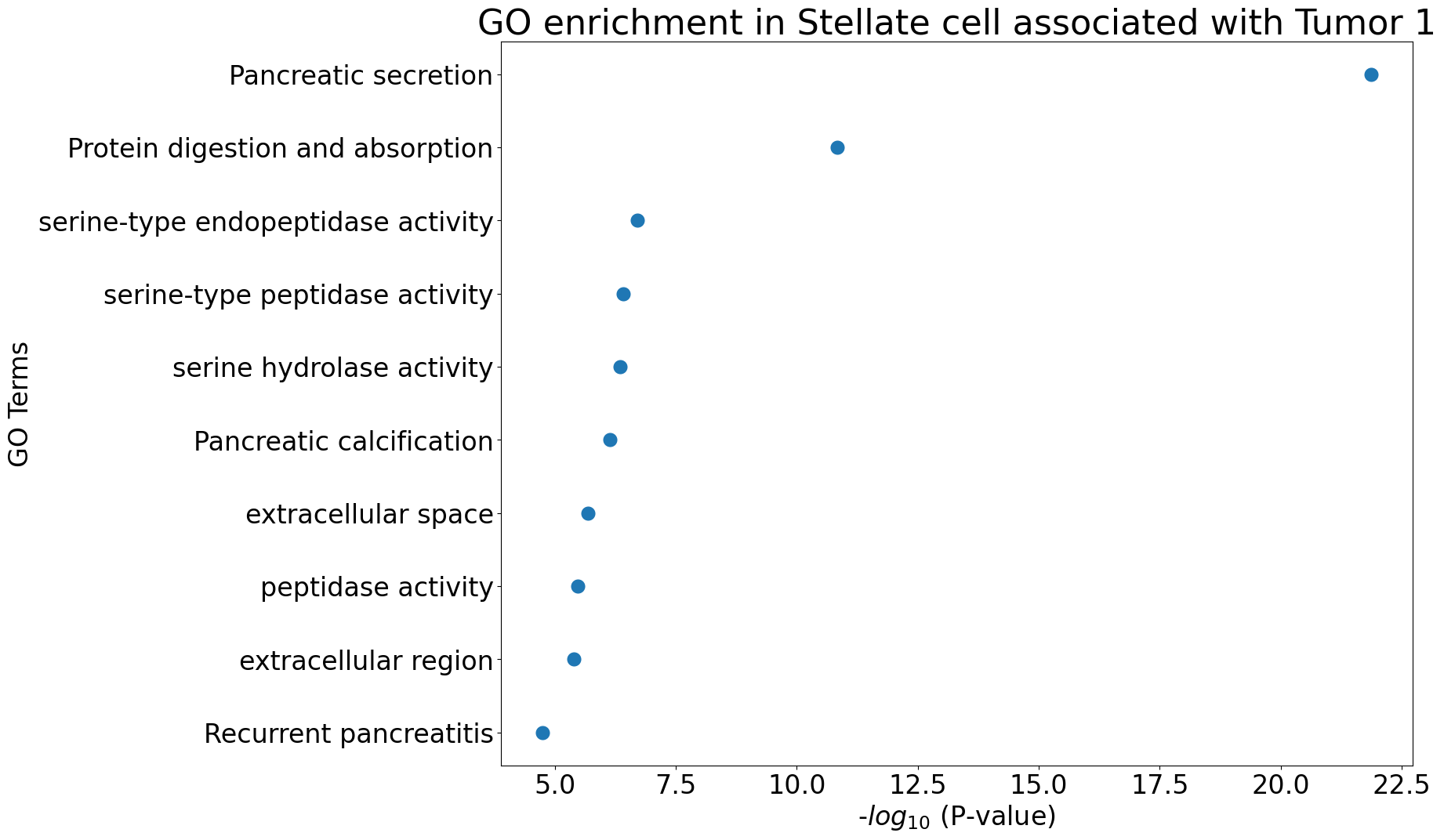
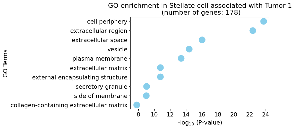
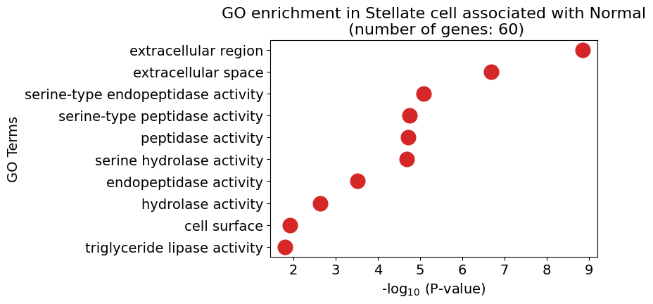
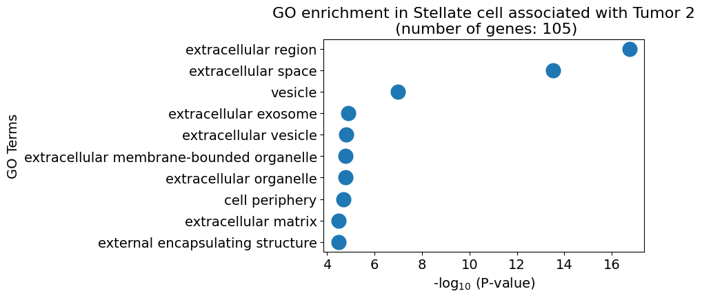
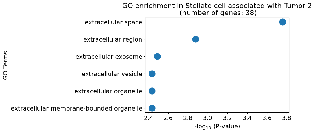
Gene Ontology analysis
pl.pl.gene_annotation_cell_type_subgroup(
    cell_type = cell_type,
    group = 'Tumor 1',
    num_gos = 10
    )
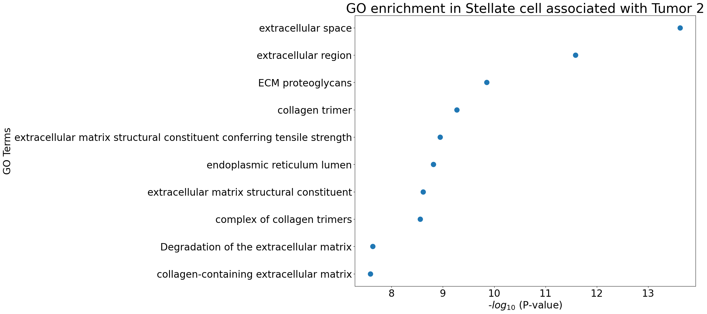
pl.pl.gene_annotation_cell_type_subgroup(
    cell_type = cell_type,
    group = 'Tumor 2',
    num_gos = 10
    )
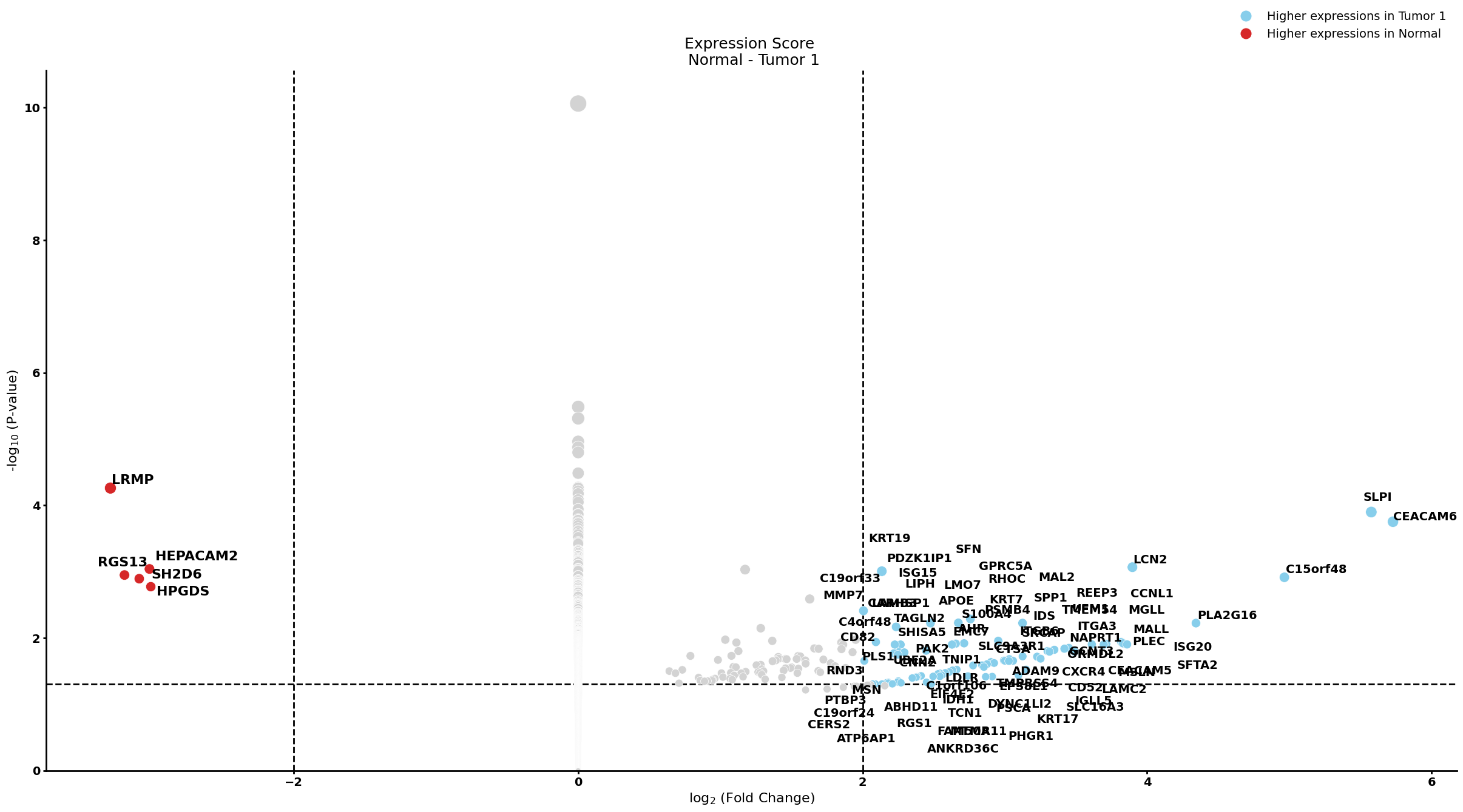
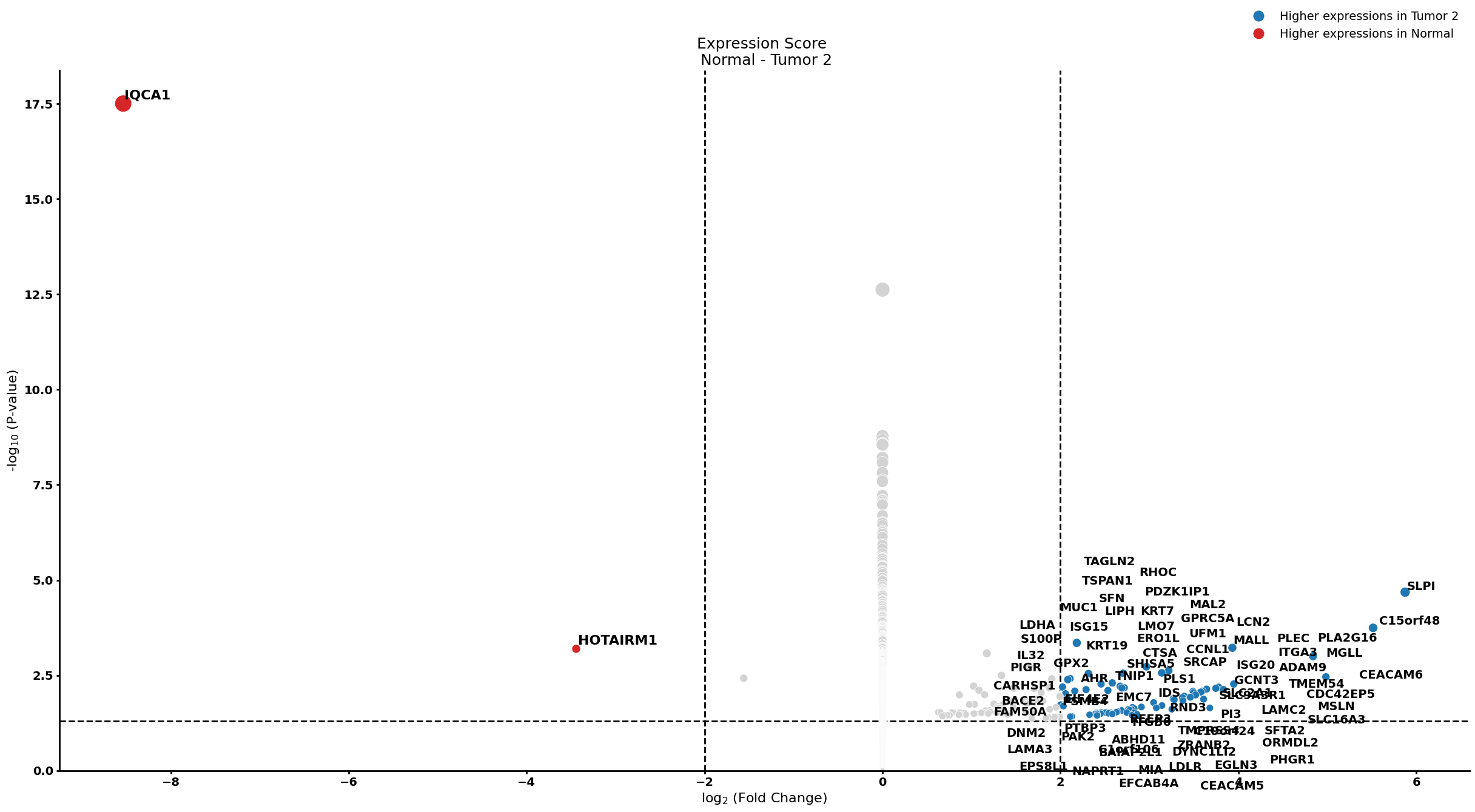
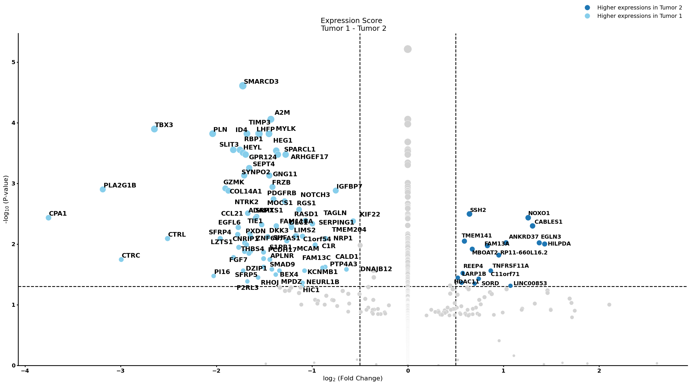
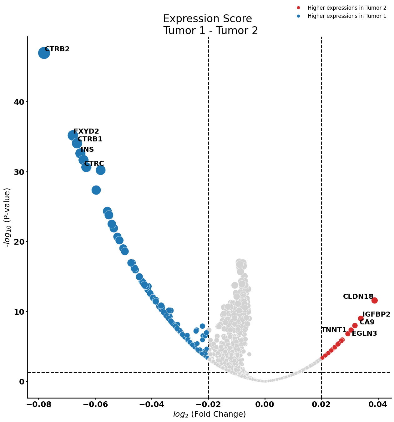
Ductal cell type 2
cell_type = "Ductal cell type 2"
pl.tl.compute_diff_expressions(
    adata,
    cell_type,
    proportion_df,
    fc_thr = 0.020,
    pval_thr = 0.05,
    group1 = 'Tumor 1',
    group2 = 'Tumor 2',
    sample_col = 'sampleID',
    col_cell = 'cell_types',
    )
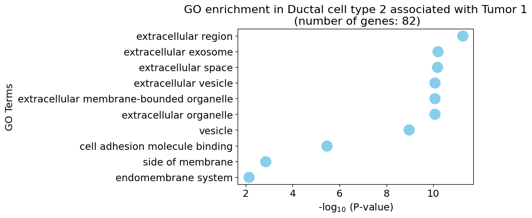
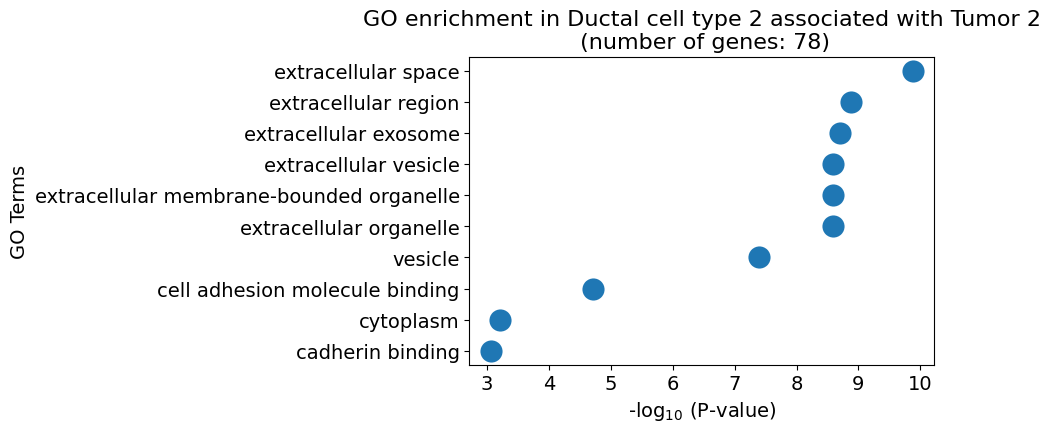
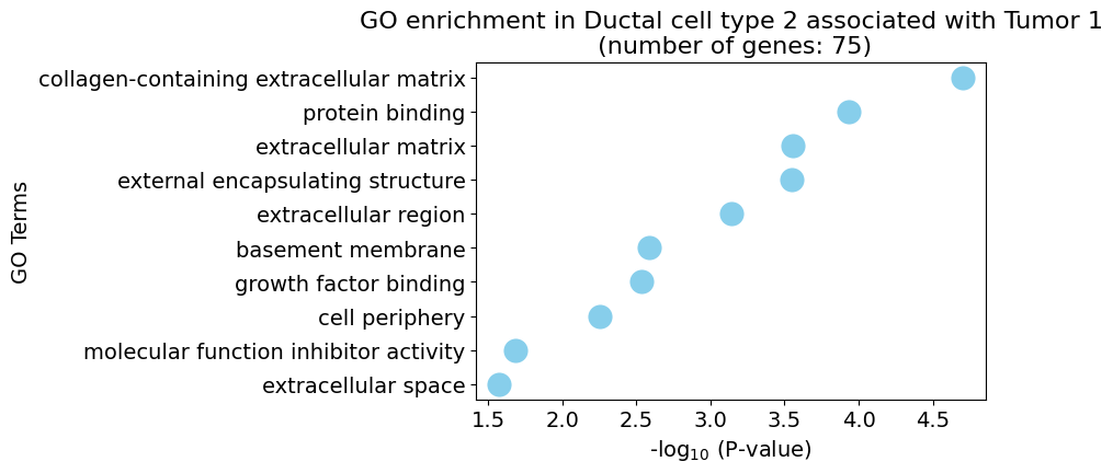
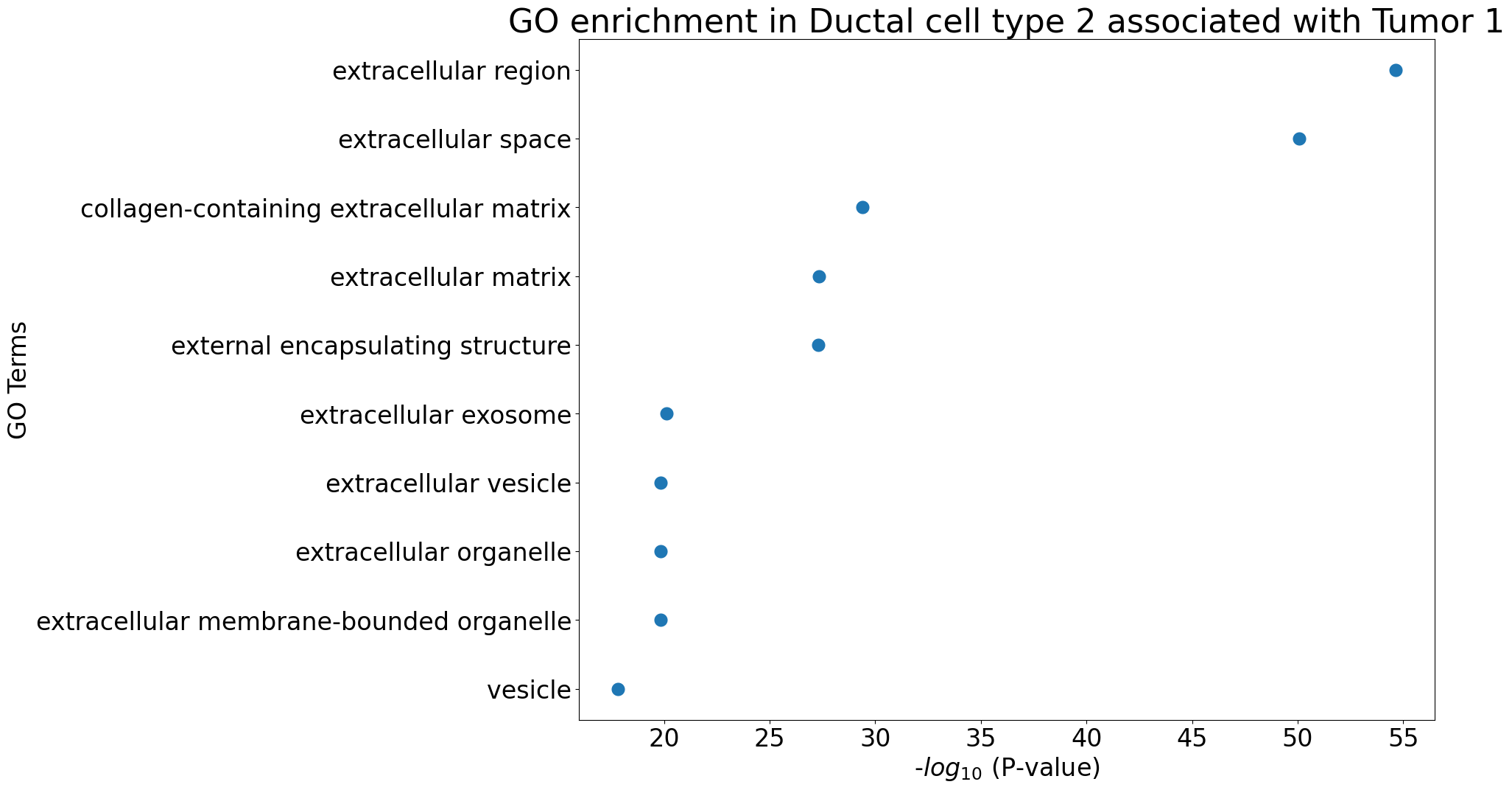
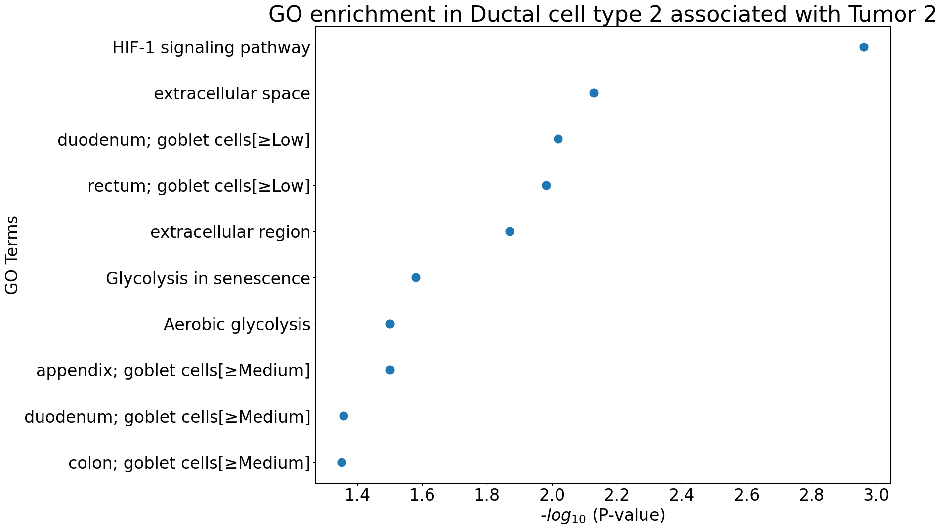
Gene Ontology analysis
pl.pl.gene_annotation_cell_type_subgroup(
    cell_type = cell_type,
    group = 'Tumor 1',
    num_gos = 10
    )
pl.pl.gene_annotation_cell_type_subgroup(
    cell_type = cell_type,
    group = 'Tumor 2',
    num_gos = 10
    )
Pseudobulk differential expression analysis
Note:
- conda install conda-forge::r-tidyverse
- conda install bioconda::bioconductor-singlecellexperiment
- conda install bioconda::bioconductor-deseq2
Stellate cell
pl.pl.get_pseudobulk_DE(adata, proportion_df, cell_type = 'Stellate cell', fc_thr = [3.0, 4.0, 0.5])
Ductal cell type 1
pl.pl.get_pseudobulk_DE(adata, proportion_df, cell_type = 'Ductal cell type 1', fc_thr = [5.0, 4.0, 0.5])
Ductal cell type 2
pl.pl.get_pseudobulk_DE(adata, proportion_df, cell_type = 'Ductal cell type 2', fc_thr = [2.0, 2.0, 0.5])